LSTM and GRU Recurrent Networks
Tinymind provides three recurrent neural network architectures for learning from sequential data: Elman (simple recurrent), LSTM (Long Short-Term Memory), and GRU (Gated Recurrent Unit). All are implemented as C++ templates and support both fixed-point and floating-point value types.
Recurrent networks maintain internal state across time steps, making them suitable for tasks like sequence prediction, time-series forecasting, and temporal pattern recognition. The key architectural difference from feed-forward networks is that hidden neurons receive feedback connections from the previous time step.
Embedded Use Cases
On resource-constrained embedded systems, recurrent networks enable on-device temporal intelligence without cloud connectivity:
- Wearable health monitoring – ECG arrhythmia detection, heart rate prediction, sleep stage classification running continuously on a battery-powered sensor
- Predictive maintenance – vibration pattern analysis on industrial equipment, detecting bearing wear or motor degradation before failure
- Sensor time-series – temperature/pressure trend prediction on IoT nodes, enabling local decision-making without network round-trips
- Embedded control – adaptive motor control, robotic joint coordination, and real-time signal processing
A trainable GRU (2->3->1) in Q8.8 fixed-point takes just 808 bytes – small enough to run on virtually any microcontroller, with no FPU, GPU, or OS required. For inference-only deployment after training in PyTorch, the memory footprint drops further to ~336 bytes.
Recurrent Network Templates
ElmanNeuralNetwork
The simplest recurrent architecture. A single hidden layer receives feedback from its own output at the previous time step. Recurrent connection depth is fixed to 1.
template<
    typename ValueType,
    size_t NumberOfInputs,
    size_t NumberOfNeuronsInHiddenLayer,
    size_t NumberOfOutputs,
    typename TransferFunctionsPolicy,
    bool IsTrainable = true,
    size_t BatchSize = 1,
    outputLayerConfiguration_e OutputLayerConfiguration = FeedForwardOutputLayerConfiguration
>
class ElmanNeuralNetwork
The Temporal XOR example (elman_temporal_xor.cpp) shows what the recurrent connection buys: trained to predict x[t] XOR x[t-1] from a stream that only ever exposes x[t], the Elman network reaches ~98% while a feed-forward MLP of the same shape — having no memory of x[t-1] — is stuck at chance.
LstmNeuralNetwork
LSTM networks use 4 gates (input, forget, output, cell candidate) to control information flow. This allows them to learn long-term dependencies that simple recurrent networks struggle with. LSTM supports multi-layer configurations via HiddenLayers<N0, N1, ...>.
template<
    typename ValueType,
    size_t NumberOfInputs,
    typename HiddenLayersDescriptor,
    size_t NumberOfOutputs,
    typename TransferFunctionsPolicy,
    bool IsTrainable = true,
    size_t BatchSize = 1,
    size_t RecurrentConnectionDepth = 1,
    outputLayerConfiguration_e OutputLayerConfiguration = FeedForwardOutputLayerConfiguration
>
class LstmNeuralNetwork
GruNeuralNetwork
GRU networks use 3 gates (update, reset, candidate) – simpler than LSTM’s 4 gates. GRU uses ~25% less memory per hidden neuron than LSTM while achieving comparable performance on many tasks. GRU is often preferred for resource-constrained embedded systems.
template<
    typename ValueType,
    size_t NumberOfInputs,
    typename HiddenLayersDescriptor,
    size_t NumberOfOutputs,
    typename TransferFunctionsPolicy,
    bool IsTrainable = true,
    size_t BatchSize = 1,
    size_t RecurrentConnectionDepth = 1,
    outputLayerConfiguration_e OutputLayerConfiguration = FeedForwardOutputLayerConfiguration
>
class GruNeuralNetwork
Template Parameters
ValueType - The numeric type used by the network. Can be a QValue fixed-point type, float, or double.
NumberOfInputs - Number of input neurons.
HiddenLayersDescriptor - Specifies hidden layer sizes. Use HiddenLayers<N> for a single hidden layer with N neurons, or HiddenLayers<N0, N1, ...> for multiple hidden layers with different sizes.
NumberOfOutputs - Number of output neurons.
TransferFunctionsPolicy - Policy class providing activation functions, random number generation, optimizer, error calculation, gradient clipping, weight decay, and learning rate schedule.
IsTrainable - When false, training code is omitted entirely, reducing binary size. Non-trainable networks can still load pre-trained weights.
BatchSize - Number of samples to accumulate before back-propagation.
RecurrentConnectionDepth - Number of previous time steps stored in recurrent connections.
OutputLayerConfiguration - FeedForwardOutputLayerConfiguration for regression, ClassifierOutputLayerConfiguration for softmax classification.
Hidden Layer Configuration
Tinymind supports heterogeneous hidden layer sizes using the HiddenLayers variadic template:
// Single hidden layer with 16 neurons
typedef tinymind::LstmNeuralNetwork<ValueType, 1,
    tinymind::HiddenLayers<16>, 1,
    TransferFunctionsType> SingleLayerLstm;

// Two hidden layers: 16 neurons then 8 neurons
typedef tinymind::LstmNeuralNetwork<ValueType, 2,
    tinymind::HiddenLayers<16, 8>, 1,
    TransferFunctionsType> TwoLayerLstm;

// Three hidden layers: 32 -> 16 -> 8
typedef tinymind::LstmNeuralNetwork<ValueType, 2,
    tinymind::HiddenLayers<32, 16, 8>, 1,
    TransferFunctionsType> ThreeLayerLstm;
LSTM Example: Sinusoid Prediction
This example trains an LSTM to predict the next value in a sinusoidal sequence. Source code: lstm_sinusoid.cpp.
Network Definition
typedef tinymind::QValue<8, 8, true, tinymind::RoundUpPolicy> ValueType;

typedef tinymind::FixedPointTransferFunctions<
    ValueType,
    RandomGen<ValueType>,
    tinymind::TanhActivationPolicy<ValueType>,
    tinymind::SigmoidActivationPolicy<ValueType>,
    1,
    tinymind::DefaultNetworkInitializer<ValueType>,
    tinymind::MeanSquaredErrorCalculator<ValueType, 1>,
    tinymind::ZeroToleranceCalculator<ValueType>,
    tinymind::GradientClipByValue<ValueType>> TransferFunctionsType;

typedef tinymind::LstmNeuralNetwork<
    ValueType, 1,
    tinymind::HiddenLayers<16>,
    1,
    TransferFunctionsType> LstmNetworkType;
Training Loop
LstmNetworkType lstmNet;
ValueType input[1], target[1], error;

for (unsigned epoch = 0; epoch < TRAINING_EPOCHS; ++epoch)
{
    for (size_t t = 0; t < NUM_SAMPLES - 1; ++t)
    {
        input[0] = sinSamples[t];
        target[0] = sinSamples[t + 1];

        lstmNet.feedForward(&input[0]);
        error = lstmNet.calculateError(&target[0]);

        if (!TransferFunctionsType::isWithinZeroTolerance(error))
        {
            lstmNet.trainNetwork(&target[0]);
        }
    }
}
Building The Example
cd examples/lstm_sinusoid
make        # debug build
make release # optimized build
cd output
./lstm_sinusoid
Floating-Point vs Q16.16
A companion example, lstm_sinusoid_float.cpp, trains the same LSTM twice on this task — once with ValueType = double, once with QValue<16, 16> — from identical seeds and inits, and overlays both on one chart. It is the only example that runs a recurrent network in floating-point. In free-run the float net holds the oscillation across both periods while the Q16.16 net collapses in the second, making the quantization cost visible directly. See the LSTM Sinusoid (Float vs Q16.16) example page.
GRU Example: XOR
This example trains a GRU to predict the XOR function with early stopping. Source code: gru_xor.cpp.
Training With Early Stopping
GruNetworkType gruNet;
tinymind::EarlyStopping<ValueType, 5000> stopper;

for (unsigned i = 0; i < TRAINING_ITERATIONS; ++i)
{
    generateXorValues(values[0], values[1], output[0]);

    gruNet.feedForward(&values[0]);
    error = gruNet.calculateError(&output[0]);

    if (!TransferFunctionsType::isWithinZeroTolerance(error))
    {
        gruNet.trainNetwork(&output[0]);
    }

    if (stopper.shouldStop(error))
    {
        break; // converged, stop training early
    }
}
Size Comparison
| Architecture | Hidden | Trainable (double) | Trainable (Q8.8) | Non-trainable (Q8.8) |
|---|---|---|---|---|
| MLP (2->5->1) | 5 | 1,008 bytes | 328 bytes | 144 bytes |
| Elman (2->3->1) | 3 | 1,056 bytes | 472 bytes | 192 bytes |
| LSTM (2->3->1) | 3 | 3,024 bytes | 952 bytes | 384 bytes |
| GRU (2->3->1) | 3 | 2,400 bytes | 808 bytes | 336 bytes |
GRU uses ~25% less memory than LSTM (3 gates vs 4 gates). Even a trainable LSTM in Q8.8 fixed-point fits in under 1 KB.
Resetting State
Recurrent networks accumulate internal state across time steps. When starting a new sequence, reset the state:
lstmNet.resetState();  // clears cell state and hidden state
gruNet.resetState();   // clears hidden state
Weight Import/Export
Trained recurrent network weights can be saved and loaded using RecurrentNetworkPropertiesFileManager:
typedef tinymind::RecurrentNetworkPropertiesFileManager<LstmNetworkType> FileManager;

// Save weights
std::ofstream outFile("lstm_weights.txt");
FileManager::storeNetworkWeights(lstmNet, outFile);

// Load weights
std::ifstream inFile("lstm_weights.txt");
FileManager::template loadNetworkWeights<ValueType, ValueType>(lstmNet, inFile);
See the Weight Import Export and PyTorch Interoperability page for details on the weight file format and PyTorch export scripts.
Liquid Neural Networks (Continuous-Time)
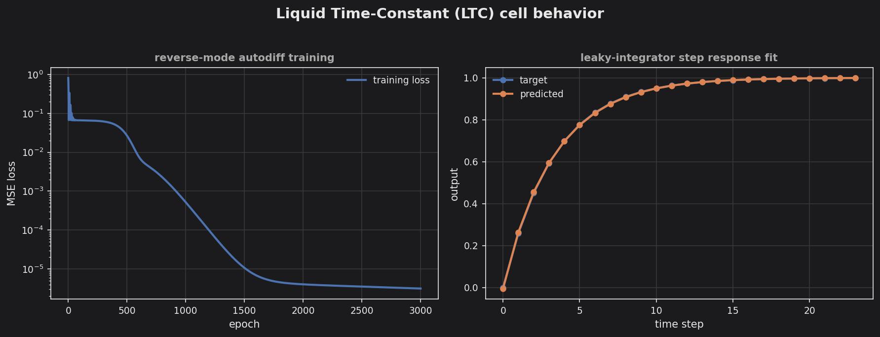
Beyond the gated RNNs above, TinyMind ships two continuous-time recurrent cells from the MIT liquid-network line of work. Instead of a discrete gate update, a liquid cell models each neuron as an ODE whose effective time constant depends on the input — well suited to irregularly-sampled time series (sensors that report at varying intervals, event streams). Both are standalone single-step cells: the caller owns the state buffer and the time loop, exactly like QLSTMCell / QGRUCell.
The float cells are written scalar-templated in the PINN style (step<S>), so the one forward pass serves double / float / fixed-point QValue inference and differentiates through the existing autodiff types (Dual, MultiDual, RevVar). They therefore train through the existing reverse-mode trainer pinn::sgdStepReverse with no hand-written backprop.
LtcCell (Liquid Time-Constant)
LtcCell<NumInputs, NumState, Act> (cpp/ltc.hpp) — the fused (semi-implicit Euler) ODE solver from Hasani et al., Liquid Time-constant Networks (AAAI 2021). Per-neuron dynamics:
dx_i/dt = -[ 1/tau_i + f_i(x, I) ] * x_i + f_i(x, I) * A_i
f_i      = Act( W_in[i,:] . I + W_rec[i,:] . x + b_i )
The fused step advances in closed form with no inner iteration and is unconditionally stable (denominator > 1) for dt, tau > 0:
x_i(t+dt) = ( x_i + dt * f_i * A_i ) / ( 1 + dt * ( 1/tau_i + f_i ) )
Reverse-mode training is enabled with -DTINYMIND_LTC_REVERSE_TRAINING=1. LTC’s continuous 1/tau dynamics stay in the float / fixed-point tiers (they resist int8); CfC is the int8-deployable liquid cell.
CfCCell (Closed-form Continuous-time)
CfCCell<NumInputs, NumState, BackboneDim, ...> (cpp/cfc.hpp) — the solver-free sibling from Hasani et al., Closed-form continuous-time neural networks (Nature MI 2022). A backbone trunk over [input ++ h_prev] feeds two tanh heads and a time-gate, interpolated by the gate:
x1   = tanh( W_bx . input + W_bh . h_prev + b_b )
ff1  = tanh( W1 . x1 + b1 )
ff2  = tanh( W2 . x1 + b2 )
t    = sigmoid( (W_A . x1) * ts + (W_B . x1) + b_time )
h'   = (1 - t) * ff1 + t * ff2
The per-step elapsed time ts is a runtime scalar feeding the time-gate, so irregular sampling is handled directly. Reverse-mode training is enabled with -DTINYMIND_CFC_REVERSE_TRAINING=1.
The examples/ltc_sequence/ and examples/cfc_sequence/ demos train each cell + a linear readout through pinn::sgdStepReverse — the CfC demo feeds a varying ts per step.
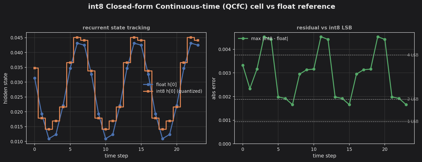
The int8 examples/qcfc_liquid_int8/ deployment exemplar tracks the float reference within ~2% of the hidden state’s dynamic range — a few int8 LSBs. See the Example Gallery for more.
Int8 Quantized Counterparts
For inference-only deployment that does not need the trainable Q-format pipeline at all, TinyMind ships pure-integer int8 cells alongside LstmNeuralNetwork / GruNeuralNetwork:
QLSTMCell— four gates (i, f, g, o) in TFLite ordering. Two rescalers per gate (input-MAC + recurrent-MAC) into a shared sigmoid / tanh LUT input scale; cell update via twomultiplyByQuantizedMultipliercalls. Cell-state storageint8_t(default) orint16_tfor long unroll horizons (gateTINYMIND_ENABLE_INT16_ACCUM=1).QGRUCell— three gates (r, z, n) in canonical ordering. Reset-before-multiply formulation,(1 - z_t)computed exactly in the sigmoid grid as-z_t.QCfCCell— int8 closed-form continuous-time (liquid) cell. Backbone trunk + two tanh heads + a sigmoid time-gate + the(1 - t) * ff1 + t * ff2interpolation; the elapsed timetsis folded into the time-gate-A requantizer at calibration (regular-sampling deployable form). Reuses the QGRU(1 - t) == 128 - tsigmoid-grid identity.
All are single-step cells; the caller owns the time loop and the hidden / cell state buffers. See Int8 Affine Quantization for the full int8 layer family and buildQLSTMParams / buildQGRUParams / buildQCfCParams host-side calibration helpers.