Network Instance Size Comparison

All Architectures: MLP vs LSTM vs GRU vs KAN

Using double (2->N->1)

Instance sizes in bytes for XOR-class network configurations using double as the value type.

Architecture	Hidden Neurons	Trainable	Non-trainable	Training Overhead
MLP (2->5->1)	5	1,008 bytes	360 bytes	+648 bytes (+180%)
Elman RNN (2->3->1)	3	1,056 bytes	384 bytes	+672 bytes (+175%)
LSTM (2->3->1)	3	3,024 bytes	960 bytes	+2,064 bytes (+215%)
GRU (2->3->1)	3	2,400 bytes	792 bytes	+1,608 bytes (+203%)
KAN (2->5->1, G=5, k=1)	5	4,208 bytes	1,256 bytes	+2,952 bytes (+235%)

Using Q8.8 Fixed-Point (XOR Configuration)

Instance sizes in bytes for XOR network configurations using QValue<8,8,true> (signed Q8.8 fixed-point, 2 bytes per value).

Architecture	Hidden Neurons	Trainable	Non-trainable	Training Overhead
MLP (2->3->1)	3	328 bytes	144 bytes	+184 bytes (+128%)
Elman RNN (2->3->1)	3	472 bytes	192 bytes	+280 bytes (+146%)
LSTM (2->3->1)	3	952 bytes	384 bytes	+568 bytes (+148%)
GRU (2->3->1)	3	808 bytes	336 bytes	+472 bytes (+140%)
KAN (2->5->1, G=5, k=1)	5	1,192 bytes	416 bytes	+776 bytes (+187%)

Relative Size (vs MLP)

	Trainable	Non-trainable
double
Elman / MLP	1.0x	1.1x
LSTM / MLP	3.0x	2.7x
GRU / MLP	2.4x	2.2x
KAN / MLP	4.2x	3.5x
Q8.8
Elman / MLP	1.4x	1.3x
LSTM / MLP	2.9x	2.7x
GRU / MLP	2.5x	2.3x
KAN / MLP	3.6x	2.9x

GRU vs LSTM

	Trainable	Non-trainable
double: GRU / LSTM	79%	83%
Q8.8: GRU / LSTM	85%	88%

GRU uses 3 gates (update, reset, candidate) versus LSTM’s 4 gates (input, forget, output, cell candidate), saving ~15-21% memory per hidden neuron.

Why Each Architecture is Larger

• MLP: One weight per connection. Minimal storage.
• Elman RNN: Same connection weights as MLP, plus a recurrent layer that stores previous hidden outputs and feeds them back as additional inputs.
• LSTM: 4 gates (input, forget, output, cell) multiply connection weights by 4x, plus recurrent state and cell memory.
• GRU: 3 gates (update, reset, candidate) multiply connection weights by 3x, plus recurrent state. ~20% smaller than LSTM.
• KAN: Each edge stores B-spline coefficients (GridSize + SplineDegree = 6 per edge with G=5, k=1), plus a base weight and spline weight. Training adds gradient, delta weight, and previous delta weight for every learnable parameter.

All architectures remain well under 1.2 KB in Q8.8 fixed-point even in trainable form, making them suitable for embedded deployment.

Liquid Cells (Continuous-Time): LTC & CfC

The liquid cells (LtcCell, CfCCell) are measured on a different basis from the rows above. The MLP/LSTM/GRU/KAN figures are sizeof(network object) — self-contained objects that embed weights and training state. The liquid cells are pointer-shaped structs over a caller-owned flat parameter array; the trainable footprint is the parameter array itself (NumParams × sizeof(ValueType)), and the optimizer state (momentum velocity, the host-only autodiff tape) lives outside the cell. The numbers below are therefore parameter bytes — the weights you store and ship — not object sizeof, so they are not directly comparable to the LSTM/GRU rows.

Each configuration below includes a small linear readout (NumState -> 1, NumState + 1 params) so the totals match a usable sequence-to-scalar model.

Cell (config)	Cell params	+ readout	Total params	Q8.8	double
LTC LtcCell<2,3>	24	4	28	56 bytes	224 bytes
CfC CfCCell<2,3,4>	84	4	88	176 bytes	704 bytes
LTC LtcCell<4,8>	120	9	129	258 bytes	1,032 bytes
CfC CfCCell<4,8,16>	752	9	761	1,522 bytes	6,088 bytes

• LTC NumParams = W_in (NumState·NumInputs) + W_rec (NumState²) + b/tau/A (3·NumState). For <2,3>: 6 + 9 + 9 = 24.
• CfC NumParams = W_bx (BackboneDim·NumInputs) + W_bh (BackboneDim·NumState) + b_b (BackboneDim) + 4·(NumState·BackboneDim + NumState) for the two tanh heads plus the time-gate A/B. For <2,3,4>: 8 + 12 + 4 + 4·15 = 84. The backbone trunk and four heads make CfC heavier than a same-width LTC or GRU — it buys the closed-form (solver-free) rollout and the per-step ts time-gate.

int8 deployable CfC (QCfCCell)

For the pure-integer deployment path the weights are int8 (1 byte each) and the biases are int32. For QCfCCell<...,2,3,4>: 68 weight bytes (8 + 12 + 48) + 52 bias bytes (13 × int32) = 120 bytes of caller-owned parameters, plus the two 256-entry int8 sigmoid/tanh LUTs (512 bytes) that are shared across every cell and layer in the model. No <cmath>, no float state on the inference path.

Signal Processing Pipeline Sizes

Instance sizes in bytes for Conv1D, Pool1D, and Dropout layers. These are standalone composable layers that sit outside the neural network template.

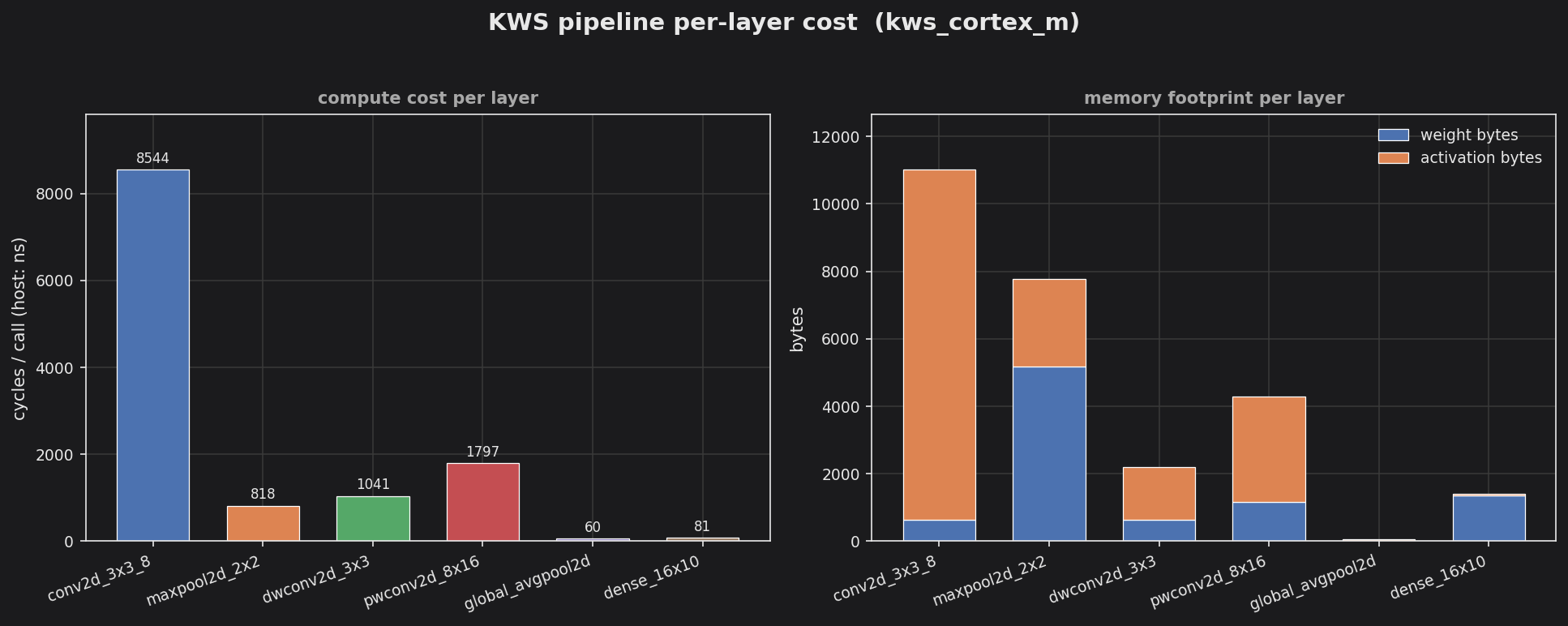
examples/kws_cortex_m (make csv && make plot): per-layer compute cost and stacked weight/activation footprint for a keyword-spotting pipeline.

Conv1D

Configuration	double	Q8.8
Conv1D (100, kernel=5, stride=2, 8 filters)	768 bytes	192 bytes
Conv1D (100, kernel=5, stride=1, 4 filters)	384 bytes	96 bytes

MaxPool1D

Configuration	Size (bytes)
MaxPool1D (96 input, pool=2, stride=2, 4 channels)	1,536 bytes
MaxPool1D (48 input, pool=2, stride=2, 1 channel)	192 bytes
MaxPool1D (6 input, pool=2, stride=2, 1 channel)	24 bytes

MaxPool1D stores argmax indices (size_t per output) for backpropagation gradient routing. Size is independent of value type.

AvgPool1D

AvgPool1D is stateless (1 byte). It has no per-instance storage since average gradients are computed directly from the pool size.

Dropout

Configuration	Size (bytes)
Dropout (192 elements, 50%)	193 bytes
Dropout (32 elements, 50%)	33 bytes
Dropout (5 elements, 50%)	6 bytes

Full Pipeline: Conv1D -> MaxPool1D -> Dropout

Value Type	Conv1D (100, k=5, s=1, 4 filters)	MaxPool1D (96, p=2, s=2, 4 ch)	Dropout (192, 50%)	Total
double	384 bytes	1,536 bytes	193 bytes	2,113 bytes
Q8.8	96 bytes	1,536 bytes	193 bytes	1,825 bytes

2D Layers

All 2D layers use NHWC layout. Sizes below are in float (the type used by the examples/kws_cortex_m/ runner). Q8.8 sizes are ~4x smaller.

Configuration	float
Conv2D (20x20x1, k=3, s=1, 8 filters)	640 bytes
DepthwiseConv2D (9x9x8, k=3)	640 bytes
PointwiseConv2D (7x7, 8 -> 16)	1,152 bytes
PointwiseConv2D (1x1, 16 -> 10; dense classifier)	1,360 bytes
MaxPool2D (18x18x8, pool=2, stride=2)	5,184 bytes
GlobalAvgPool2D (7x7x16)	1 byte

Conv2D / DepthwiseConv2D / PointwiseConv2D store both weights and gradients (2x overhead) to support on-device training. MaxPool2D stores size_t argmax indices per output. GlobalAvgPool2D is stateless.

Full Pipeline: Conv2D -> MaxPool2D -> DepthwiseConv2D -> PointwiseConv2D -> GlobalAvgPool2D -> Dense

Running the pipeline in examples/kws_cortex_m/ (20x20x1 input, 10 output classes, all float):

Section	Bytes
Total weight + state bytes	8,976
Peak activation buffer	10,368 (first conv output)

Swapping the layer value type from float to Q8.8 roughly quarters the Conv / DW / PW / Dense storage and halves each activation buffer. The MaxPool2D argmax array is size_t-indexed and is independent of value type – on a tight MCU target it becomes the dominant term and is the best candidate for the next round of footprint work.

Binary and Ternary Dense Layer Sizes

BinaryDense (Trainable)

Configuration	double	Q8.8
BinaryDense (4, 2)	168 bytes	44 bytes
BinaryDense (16, 8)	2,192 bytes	560 bytes
BinaryDense (64, 16)	16,768 bytes	4,288 bytes

TernaryDense (Trainable)

Configuration	double	Q8.8
TernaryDense (4, 2, 50%)	168 bytes	44 bytes
TernaryDense (16, 8, 50%)	2,208 bytes	576 bytes
TernaryDense (64, 16, 50%)	16,896 bytes	4,416 bytes

Inference-Only Packed Weight Storage

Configuration	Binary (packed)	Ternary (packed)	Full double	Full Q8.8
64x16 weights + biases	256 bytes	384 bytes	8,320 bytes	2,080 bytes
32x32 weights + biases	384 bytes	512 bytes	8,448 bytes	2,112 bytes

Weight Storage Compression Ratios (64x16 layer)

Storage	Bytes	vs double	vs Q8.8
Full double	8,192 bytes	1x	–
Full Q8.8	2,048 bytes	4x	1x
Packed binary (1-bit)	128 bytes	64x	16x
Packed ternary (2-bit)	256 bytes	32x	8x