A Neural Network in Under 4KB

To demonstrate what a tinymind neural network can do, I chose to implement a classic “hello world” kind of program for neural networks (xor.cpp). Here I will demonstrate how to instantiate and train a neural network to predict the outcome of the mathematical XOR function. We will generate and feed known data into the neural network and train it to become an XOR predictor. By inspecting the generated output file during compilation, we can prove to ourselves that the whole neural network and associated code and data occupies under 4KB in the final image, assuming we turn on compiler optimizations.

Important: that 4KB is a trainable network — it learns on the device. The figure includes the full backpropagation machinery: the code that computes gradients and updates weights, plus the extra per-connection state (gradient + current/previous delta-weight) that training needs in RAM. If you only need to run an already-trained model, you compile the network with IsTrainable=false and the entire training path drops out — the inference-only footprint is roughly a third of the trainable one. See Trainable vs. Inference-Only Footprint below for measured numbers.

What 4KB Means for Embedded

On a microcontroller like the STM32L0 (ARM Cortex-M0+) with 16 KB of flash and 2 KB of RAM, a 4KB trainable neural network consumes 25% of flash – leaving room for the application, peripherals, and communication stack. And that is the trainable figure: a deployed inference-only build (IsTrainable=false) is far smaller still, since the backprop code and the per-weight gradient/delta state both disappear.

For comparison, the minimum footprint of TensorFlow Lite Micro is ~50-100 KB – it won’t fit on this device at all, let alone leave room for anything else. Tinymind makes neural networks feasible on hardware where no other framework can run.

Q Format

To make the neural network small and fast, we can’t afford the luxury of floating point numbers. Also, when I was developing tinymind the hardware I had didn’t have a floating point unit, which makes using floating point even more difficult and expensive. We need to use fixed-point numbers to solve this problem. Tinymind contains a C++ template library to help us here, Q Format. See the Q-Format page for a full explanation of how it works.

We declare the size and resolution of our Q-Format type like this:

// Q-Format value type
static const size_t NUMBER_OF_FIXED_BITS = 16;
static const size_t NUMBER_OF_FRACTIONAL_BITS = 16;
typedef tinymind::QValue<NUMBER_OF_FIXED_BITS, NUMBER_OF_FRACTIONAL_BITS, true> ValueType;

We have now declared a signed (the template parameter true means it is signed) Q16.16 fixed-point type. The fractional part resolution is 2^(-16), about 0.0000153, which is plenty of precision to train XOR smoothly. (The original version of this example used Q8.8; the coarser 1/256 grid made the learning curve lurch through the XOR saddle point before snapping to a solution, so it was bumped to Q16.16 for a smooth, monotonic descent.) The fixed and fractional portions are concatenated into a 32-bit field. As an example, the floating point number 1.5 is represented as 0x18000 in Q16.16: the integer portion (1) is shifted up by the number of fractional bits (16) to give 0x10000, then we OR in half the fractional range (0x8000).

Neural Network

We need to specify our neural network architecture. We do it as follows:

// Neural network architecture
static const size_t NUMBER_OF_INPUTS = 2;
static const size_t NUMBER_OF_HIDDEN_LAYERS = 1;
static const size_t NUMBER_OF_NEURONS_PER_HIDDEN_LAYER = 4;
static const size_t NUMBER_OF_OUTPUTS = 1;

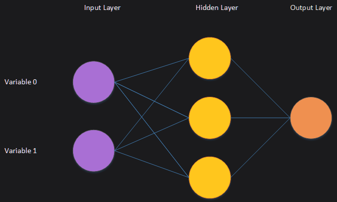
We’ll define a neural network with 2 input neurons, 1 hidden layer with 4 neurons in it, and 1 output neuron. The 2 input neurons will receive the streams of 1s and 0s from the training data. The output neuron outputs the predicted result of the operation. The hidden layer is the transfer function which learns to predict the result, given the input values and the known result.

We typedef the neural network transfer functions policy as well as the neural network itself:

// Typedef of transfer functions for the fixed-point neural network
typedef tinymind::FixedPointTransferFunctions<  ValueType,
RandomNumberGenerator,
tinymind::TanhActivationPolicy<ValueType>,
tinymind::SigmoidActivationPolicy<ValueType>> TransferFunctionsType;
// typedef the neural network itself
typedef tinymind::MultilayerPerceptron< ValueType,
NUMBER_OF_INPUTS,
NUMBER_OF_HIDDEN_LAYERS,
NUMBER_OF_NEURONS_PER_HIDDEN_LAYER,
NUMBER_OF_OUTPUTS,
TransferFunctionsType> NeuralNetworkType;

The TransferFunctionsType specifies the ValueType (our Q-format type), the random number generator for the neural network, the activation policy for Input->Hidden layers (tanh), as well as the activation policy for the Hidden->Output layer (sigmoid, so the output sits in the [0, 1] range of the XOR targets). The neural network code within tinymind makes no assumptions about its environment. It needs to be provided with template parameters which encapsulate policy.

Lookup Tables

Since the hardware I was using didn’t have a floating point unit, I also did not have the luxury of the built in math functions for tanh, sigmoid, etc. To get around this limitation, tinymind generates and utilizes lookup tables (LUTs) for these activation functions (activationTableGenerator.cpp). This generator generates header files for every supported activation function and Q-Format resolution. Because we don’t want to generate code we’re not going to use, we need to define preprocessor symbols to compile in the LUT(s) we need. If you look at the compile command you’ll see the following:

-DTINYMIND_USE_TANH_16_16=1 -DTINYMIND_USE_SIGMOID_16_16=1

This instructs the compiler to compile in the tanh and sigmoid activation LUTs for the Q-Format type Q16.16, which is what we’re using in this example (tanh for the hidden layer, sigmoid for the output layer). We need to do this for every LUT we plan to use – LUTs we don’t reference are never compiled in, so we only pay for what we use.

Generating Training Data

We’ll generate the training data programmatically. The function generateXorTrainingValue is called to generate a single training sample. We use the built-in random number generator to generate the 2 inputs:

static void generateXorTrainingValue(ValueType& x, ValueType& y, ValueType& z)
{
    const int randX = rand() & 0x1;
    const int randY = rand() & 0x1;
    const int result = (randX ^ randY);
    x = ValueType(randX, 0);
    y = ValueType(randY, 0);
    z = ValueType(result, 0);
}

We feed the data into the neural network, predict an output, and then train if we have an error outside of our zero-tolerance:

for (unsigned i = 0; i < TRAINING_ITERATIONS; ++i)
{
    generateXorTrainingValue(values[0], values[1], output[0]);
    testNeuralNet.feedForward(&values[0]);
    error = testNeuralNet.calculateError(&output[0]);
    if (!NeuralNetworkType::NeuralNetworkTransferFunctionsPolicy::isWithinZeroTolerance(error))
    {
        testNeuralNet.trainNetwork(&output[0]);
    }
    testNeuralNet.getLearnedValues(&learnedValues[0]);

Compiling The Example

To compile the example, cd to the example dir and type:

make

To make the optimized target:

make release

To clean out old outputs and force re-compile and link:

make clean

Running the Program

You can run the program by invoking:

make run

Plotting Results

After running the example, you will see a text file output, nn_fixed_xor.txt. To plot the results:

make plot

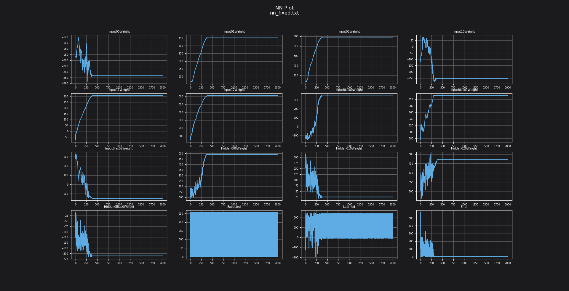
You can see the weights training through time, as well as the error reducing through time, as the predicted value approximates the expected value. The training targets map 0 and 1 onto our Q-Format type – the representation of 1.0 in a signed Q16.16 format is 0x10000 (65536), and 0.0 is 0.

Determining Neural Network Size

To determine how much space the neural network code and data occupies:

make release
size output/xornet.o output/lookupTables.o

text   data    bss    dec    hex filename
1542      8    580   2130    852 output/xornet.o
 800      0      0    800    320 output/lookupTables.o

The neural network object plus the Q16.16 tanh and sigmoid LUTs occupy roughly 2.3 KB of flash (text) – comfortably under 4KB. (bss is zero-initialized RAM; data is initialized RAM.) The exact bytes shift with compiler version and flags; the point is the order of magnitude.

Trainable vs. Inference-Only Footprint

The headline figure above is for a network that trains on the device. Backpropagation is not free: it adds the gradient-descent code path and, in RAM, three extra values per connection (the gradient and the current/previous delta-weights) that only exist while a network is learning. Set the IsTrainable template parameter to false and that entire path is compiled out – you keep feedForward and drop trainNetwork, calculateError, and the per-connection training state.

MultilayerPerceptron takes IsTrainable right after the transfer-functions policy:

// Trainable (learns on-device) -- the default
typedef tinymind::MultilayerPerceptron<ValueType, 2, 1, 4, 1, TransferFunctionsType, true>  TrainableNet;
// Inference-only (deploy a pre-trained model)
typedef tinymind::MultilayerPerceptron<ValueType, 2, 1, 4, 1, TransferFunctionsType, false> InferenceNet;

Compiling the same 2->4->1 Q16.16 network both ways (a single translation unit that instantiates the network and exercises it, g++ -O3) gives:

Build	code (text)	RAM (bss)
Trainable (feedForward + trainNetwork)	~5,180 bytes	640 bytes
Inference-only (feedForward only)	~1,730 bytes	208 bytes

Inference-only is about a third of the code and a third of the RAM. So the “under 4KB” milestone is the cost of a self-contained network that learns on the microcontroller; if you train on a host and ship only the weights, the deployed model is dramatically smaller. The usual workflow is exactly that: train (here, or in PyTorch – see the PyTorch import examples), then deploy inference-only.

Conclusion

Using tinymind, neural networks can be instantiated using fixed-point numbers so that they take up a very small amount of code and data space. I hope that this inspires you to clone tinymind and give the unit tests and examples a look. Maybe even generate one of your own.