CfC Sequence (Closed-form Continuous-time)

Trains a Closed-form Continuous-time (CfC) cell plus a linear readout to track an irregularly-sampled decaying sinusoid, feeding the varying per-step elapsed time into the cell’s time-gate.

How it works

A single CfCCell<1, 8, 16> (one input, eight state neurons, 16-unit backbone) from cpp/cfc.hpp followed by an 8-weight + bias linear readout. Inference runs in double; weights are a flat caller-owned array. Float build (TINYMIND_ENABLE_FLOAT=1, TINYMIND_ENABLE_STD=1).
Demonstrates the solver-free CfC cell: a backbone trunk, two tanh heads, and a time-gated interpolation between them, with no inner ODE iteration per step.
The headline feature is irregular sampling. Each of the 20 steps advances time by a varying delta ts that feeds the CfC time-gate, while the target is a continuous decaying sinusoid sampled at those irregular instants. The same scalar-templated step<S> supplies the RevVar training gradient and the double inference pass; training is 8000 epochs of pinn::sgdStepReverse with momentum.

Build and run

cd examples/cfc_sequence
make release
make run
make plot      # needs matplotlib; a venv/pyenv works if it is not already in your Python

make run writes cfc_loss.csv (per-epoch training loss) and cfc_fit.csv (per-step ts, target, and predicted), which plot.py reads. The example exits non-zero unless the loss at least halves. Reverse-mode training is gated by the example’s -DTINYMIND_CFC_REVERSE_TRAINING=1.

Output

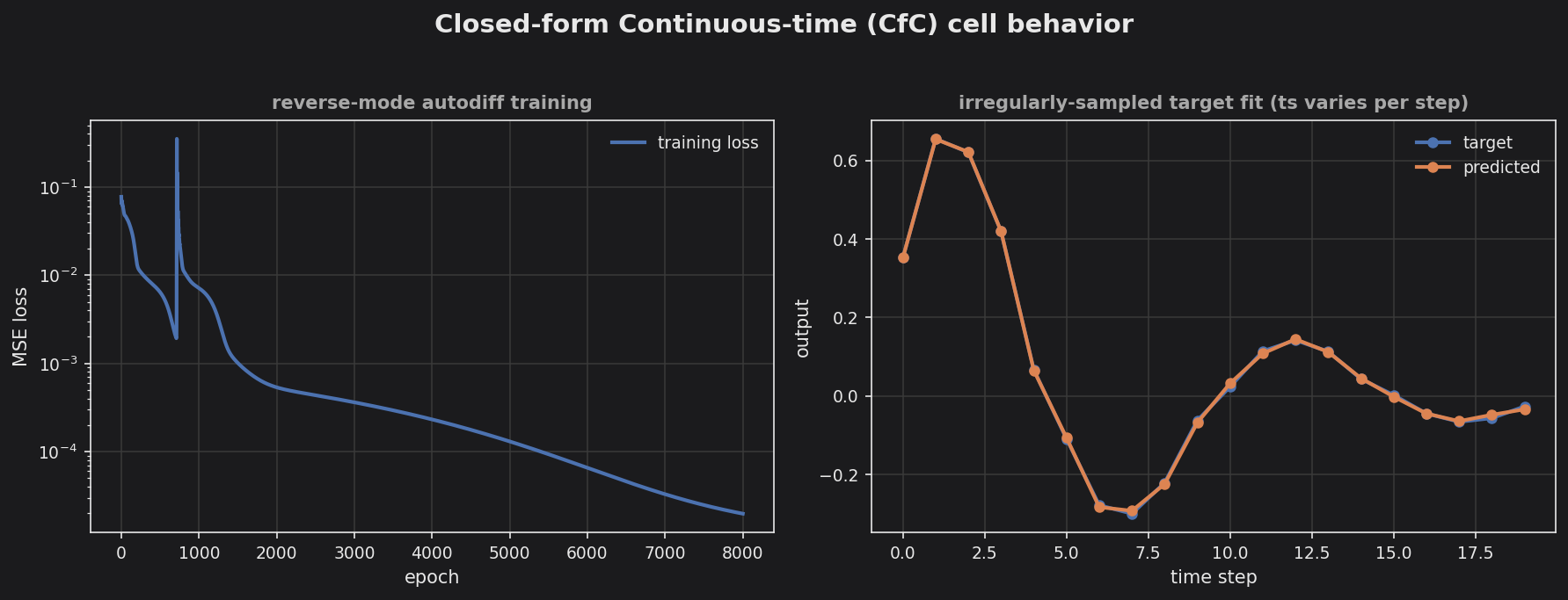
CfC training loss and irregularly-sampled target fit

The left panel shows the MSE loss decreasing across training (the early transient spike is the momentum optimizer settling). The right panel overlays the predicted output on the irregularly-sampled decaying-sinusoid target; the curves track closely, showing the CfC cell handles non-uniform time steps that a plain RNN cannot represent.

Source on GitHub