PINN: 1-D Heat Equation

A physics-informed neural network that learns the 1-D heat equation u_t = nu * u_xx by minimizing the PDE residual computed with forward-mode automatic differentiation, then re-evaluates the residual in Q16.16 fixed point for deployment.

How it works

A PinnMlp<2, 12, 1> field u(x, t): a single-hidden-layer tanh MLP with 12 units, from cpp/pinn.hpp. The autodiff and training paths run in double with std::tanh; the deployment residual benchmark runs the same field in Q16.16 fixed point (QValue<16, 16>) using the tanh lookup table (TINYMIND_USE_TANH_16_16).
Demonstrates differentiating the network with respect to its input coordinates: u_t via a first-order dual and u_xx via a nested second-order dual, the exact derivatives a PDE residual needs and that weight-gradient backprop cannot supply. Weight gradients during training come from finite differences over the exact-autodiff residual.
The residual is enforced on an interior collocation grid over x in [0, 1], t in [0, T], with the analytic reference u(x, t) = exp(-nu*pi^2*t) * sin(pi*x). After training, the residual is recomputed in fixed point so the int8/fixed-point error against the double residual is bounded, giving a fixed-point residual-accuracy benchmark.

Build and run

cd examples/pinn_heat1d
make release
make run
make plot      # needs matplotlib; a venv/pyenv works if it is not already in your Python

make run runs the verification checks (exact-solution residual, autodiff vs central finite differences, fixed-point residual benchmark). To produce the data plot.py reads, run the host-side training loop first with make train (built -O3, ~thousands of epochs but under a second), which writes pinn_loss.csv (residual loss and solution L2 error per epoch) and pinn_solution.csv (learned vs analytic field at two times). The fixed-point inference path pulls in lookupTables.cpp for the Q16.16 tanh table.

Output

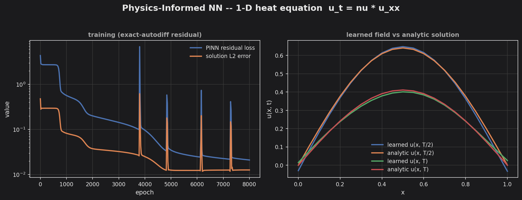
PINN heat-equation training curves and learned field vs analytic solution

The left panel shows the PINN residual loss and the solution L2 error both falling over training (the periodic spikes are optimizer transients that immediately recover). The right panel overlays the learned field on the analytic solution at T/2 and T; the learned curves match the closed-form heat-diffusion profiles closely, including the correct exponential decay of the peak between the two times.

Source on GitHub