KAN XOR
Solves the same XOR task as the classic MLP example, but with a Kolmogorov-Arnold Network (KAN) instead of a standard perceptron. The contrast highlights how KANs put the learnable non-linearity on the edges rather than fixed activations on the nodes.
How it works
- Q16.16 signed fixed-point Kolmogorov-Arnold Network (
tinymind::KolmogorovArnoldNetwork) with a 2 -> 5 -> 1 topology, a grid size of 5 and degree-1 (piecewise-linear) B-spline edges. - Demonstrates the KAN architecture in fixed point: each connection carries a learnable spline rather than a single scalar weight, and the spline coefficients are trained by backpropagation.
- Uses Q16.16 (not Q8.8) because B-spline training needs the extra range and precision; the learning-rate, momentum, and acceleration constants are tuned small to keep the spline updates stable.
Build and run
cd examples/kan_xor
make release
make run
make plot      # needs matplotlib; a venv/pyenv works if it is not already in your Python
make run runs the example twice — the default 4-corner training and --dense — writing the learning-curve CSV output/kan_xor_training.csv, the decision-surface CSV output/kan_xor_decision_surface.csv (a 41×41 sweep of the trained KAN over the input grid), the dense-training surface output/kan_xor_dense_decision_surface.csv, and a per-iteration error log output/kan_fixed_xor.txt; the plotted error is accumulated in floating point so the curve stays clean despite the fixed-point internals.
Output

The log-scale learning curve drops by roughly two orders of magnitude within the first few hundred iterations and then holds a low, stable error floor for the rest of training. This shows the piecewise-linear spline edges fit the XOR surface quickly and remain numerically stable in Q16.16 fixed point.
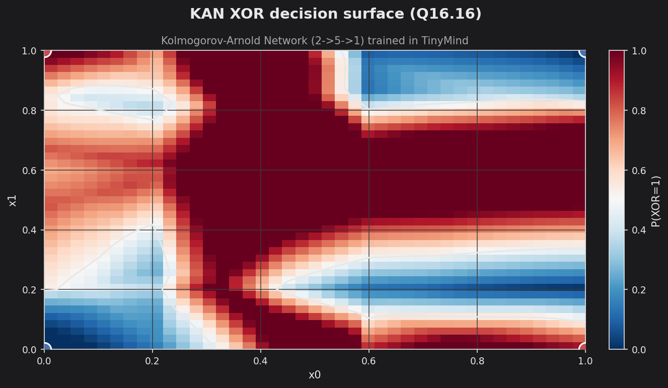
Sweeping the trained KAN over the [0,1]² input grid gives the predicted-vs-actual view: the heatmap is P(XOR=1) and the four corner markers are the ground-truth targets (red = 1, blue = 0). Every corner lands in the correct region, so all four patterns classify correctly. The busy interior is characteristic of KAN — the learnable B-spline edges are trained only on the four corner points, so they fit those exactly but extrapolate freely in between, unlike the smoother sigmoid-MLP surfaces of the fixed-point and PyTorch XOR examples.
KAN trained on dense samples
The busy surface above is not a limitation of KANs — it is the consequence of constraining ~60 spline coefficients with only 4 data points. A KAN classifier is normally trained over its whole input region, not on isolated points. Run ./output/kan_xor --dense to train the same 2->5->1 network on samples drawn uniformly from [0,1]² (labelled by the XOR of the two halves):
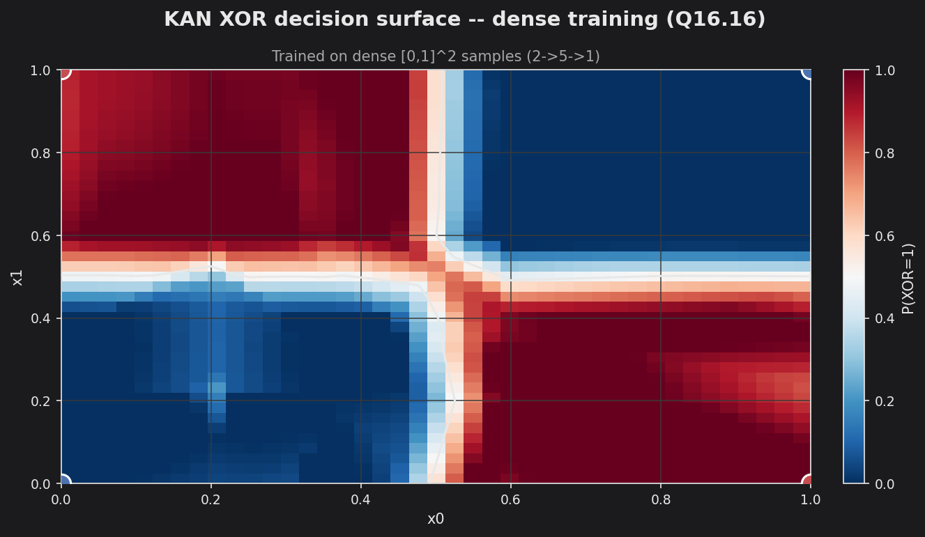
Now the splines are constrained everywhere and the network recovers the clean four-quadrant XOR map: P(XOR=1) is high in the top-left and bottom-right quadrants and low in the other two, with a sharp boundary along x0 = 0.5 and x1 = 0.5. This is the same KAN, same grid (GRID_SIZE=5) and same piecewise-linear edges (SPLINE_DEGREE=1) — only the training distribution changed. The lesson: KAN’s local-spline basis has a weaker built-in smoothness prior than a tanh MLP, so it needs data across the region (or a coarser grid / regularization) to produce a smooth surface; given that, it generalizes as cleanly as the MLP and GRU.