XOR (fixed-point MLP)
Trains a small multilayer perceptron to learn the classic non-linearly-separable XOR function, the canonical “hello world” of neural networks. The four XOR cases are generated on the fly and the network is trained purely in fixed-point arithmetic.
How it works
- Q16.16 signed fixed-point MLP with a 2 -> 4 -> 1 topology (
tinymind::MultilayerPerceptron), tanh hidden activation and sigmoid output. - Demonstrates that backpropagation converges in pure fixed-point with no FPU: weights, activations, and gradients are all
QValue<16, 16>. (The original Q8.8 / 3-neuron build worked but lurched through the XOR saddle-point plateau before snapping to a solution; Q16.16 with a 4-neuron hidden layer descends smoothly.) - A deterministic validation pass over the four canonical XOR cases (0/0, 0/1, 1/0, 1/1) is logged every 100 iterations, giving a clean convergence signal instead of the noisy random-sample error.
Build and run
cd examples/xor
make release
make run
make plot      # needs matplotlib; a venv/pyenv works if it is not already in your Python
make run writes the learning-curve CSV output/xor_training.csv, the decision-surface CSV output/xor_decision_surface.csv (a 41×41 sweep of the trained network over the input grid), and a per-iteration property dump output/nn_fixed_xor.txt. A make plot-trajectory target renders the generic per-column network-trajectory view from the property dump.
Output
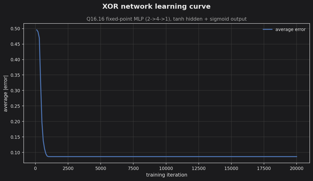
The curve plots the mean absolute error over the four XOR cases against training iteration. It descends smoothly from the symmetric-guess level (~0.5) and settles within ~1000 iterations. All four patterns are then classified correctly with clear margins (predictions ≈ 0.09 / 0.91); the residual ~0.09 is just the sigmoid output not fully saturating to 0/1 under the MSE objective.
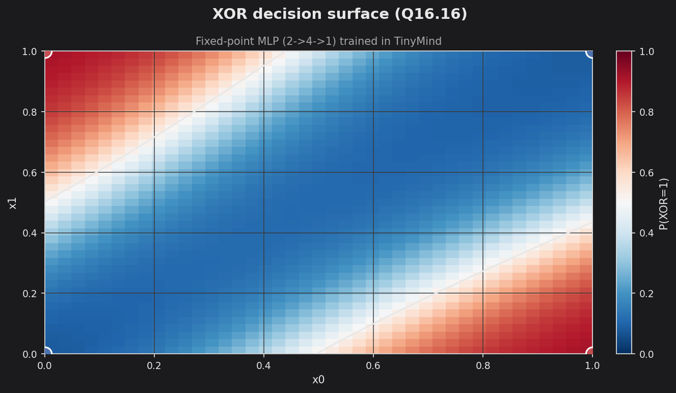
Sweeping the trained network over the [0,1]² input grid shows predicted vs. actual directly: the heatmap is the network’s P(XOR=1), the black line is the 0.5 decision boundary, and the four corner markers are the ground-truth XOR targets (red = 1, blue = 0). Each corner sits firmly inside the matching colored region — the same predicted-vs-actual view as the PyTorch Q-format and PyTorch int8 XOR examples.