Example Gallery

Every runnable example in examples/ writes a header-row CSV to its output/ directory and ships a plot.py that renders the network’s behavior. Reproduce any graph below with:

cd examples/<name> && make run && make plot   # writes output/*.csv and a PNG

The plot scripts share one style module, examples/plotting/tinymind_plot.py (matplotlib only, headless-safe). The CSV-first contract means you can also drop the data into pandas / a spreadsheet and build your own visualizations.

The graphs below use the dark theme to match this site; make plot defaults to a light theme (readable on any viewer). Set TINYMIND_PLOT_THEME=dark to reproduce these exactly.

Training dynamics

XOR learning curve — Q16.16 fixed-point MLP (2→4→1).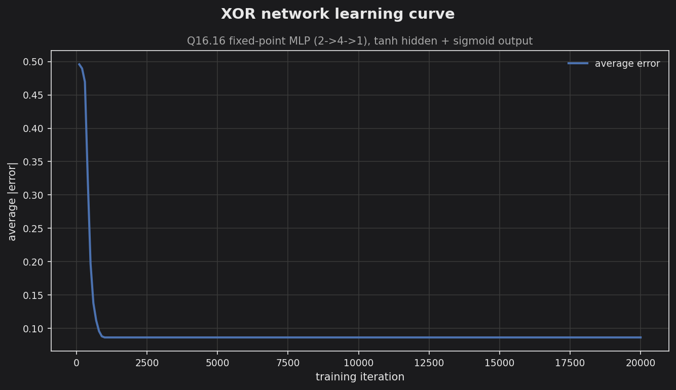

KAN XOR learning curve — Kolmogorov-Arnold network with learnable B-spline edges.

Liquid neural networks (continuous-time)

LTC — fused ODE-solver cell trained to a leaky-integrator step response via reverse-mode autodiff.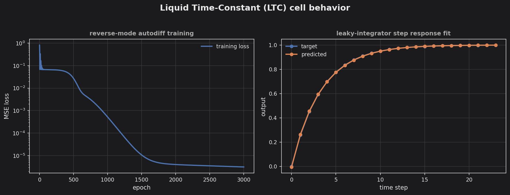

CfC — closed-form continuous-time cell on an irregularly-sampled target (per-step ts into the time-gate).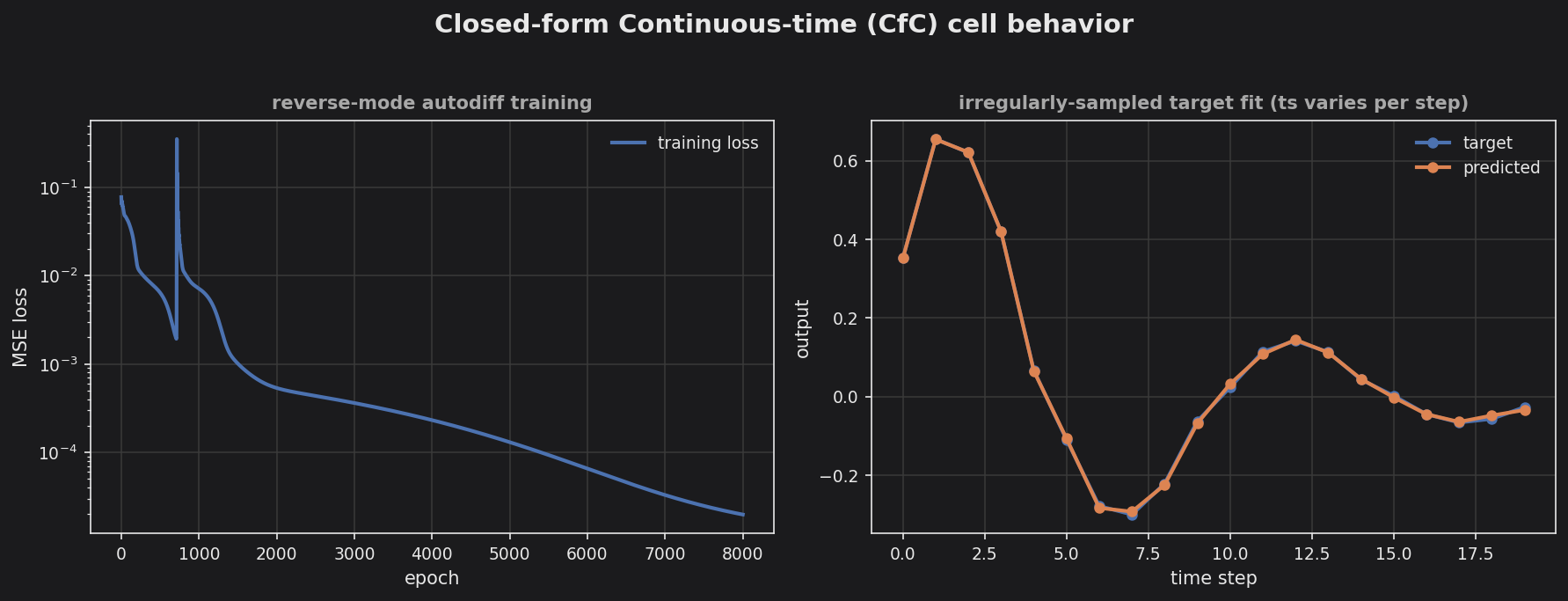

int8 QCfC — pure-integer CfC cell tracking the float reference, with per-step quantization error.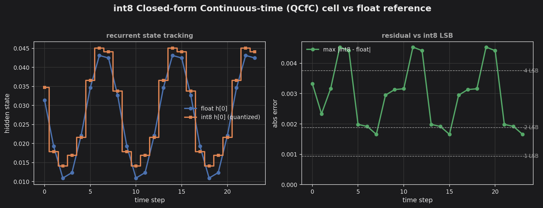

Physics-Informed NN

1-D heat equation — exact-autodiff residual training + learned field vs the analytic solution.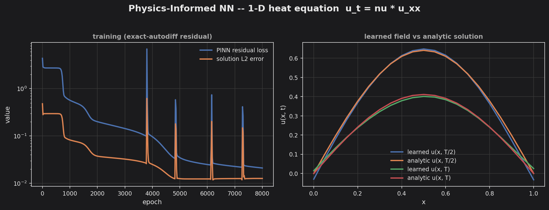

int8 quantization parity

Transformer encoder block (int8) — int8 vs float output overlay + per-element quantization error.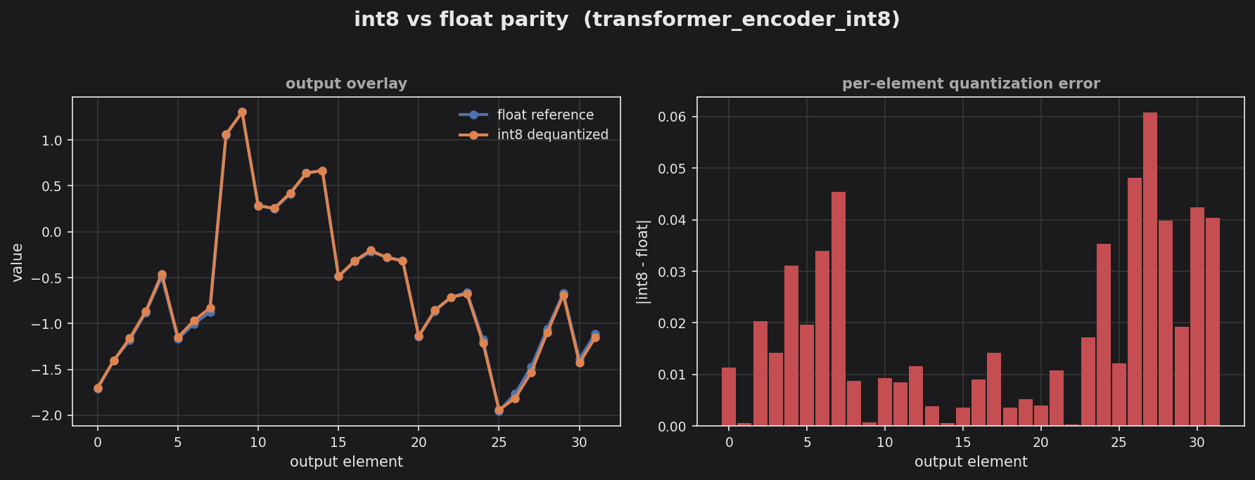

Transformer encoder stack (int8) — token embedding + sinusoidal positional encoding + 2 stacked linear-attention blocks, end-to-end.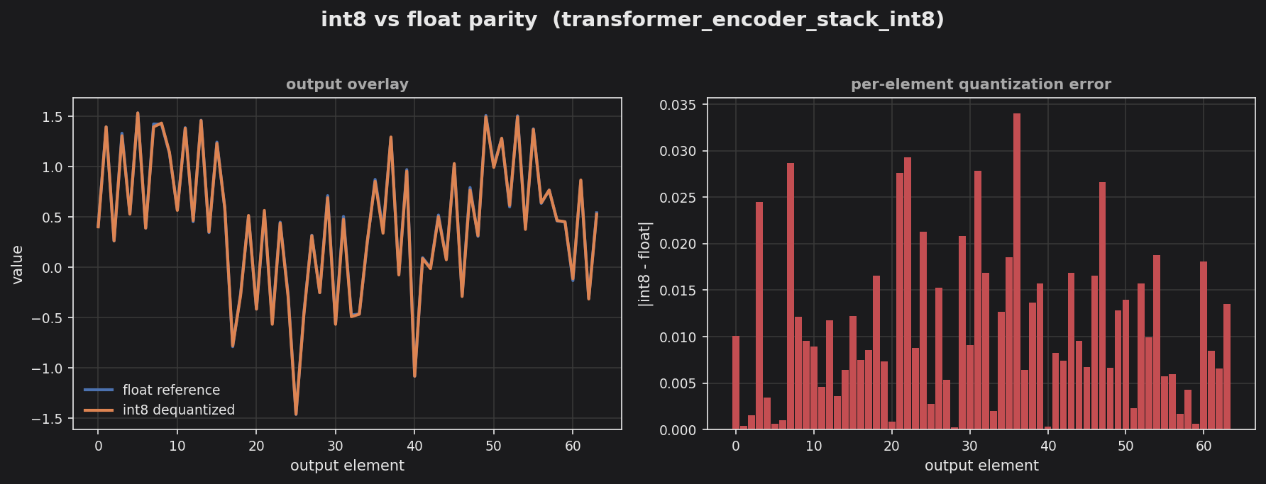

Transformer encoder stack, softmax attention (int8) — same stack with standard softmax self-attention (score grid + exp LUT).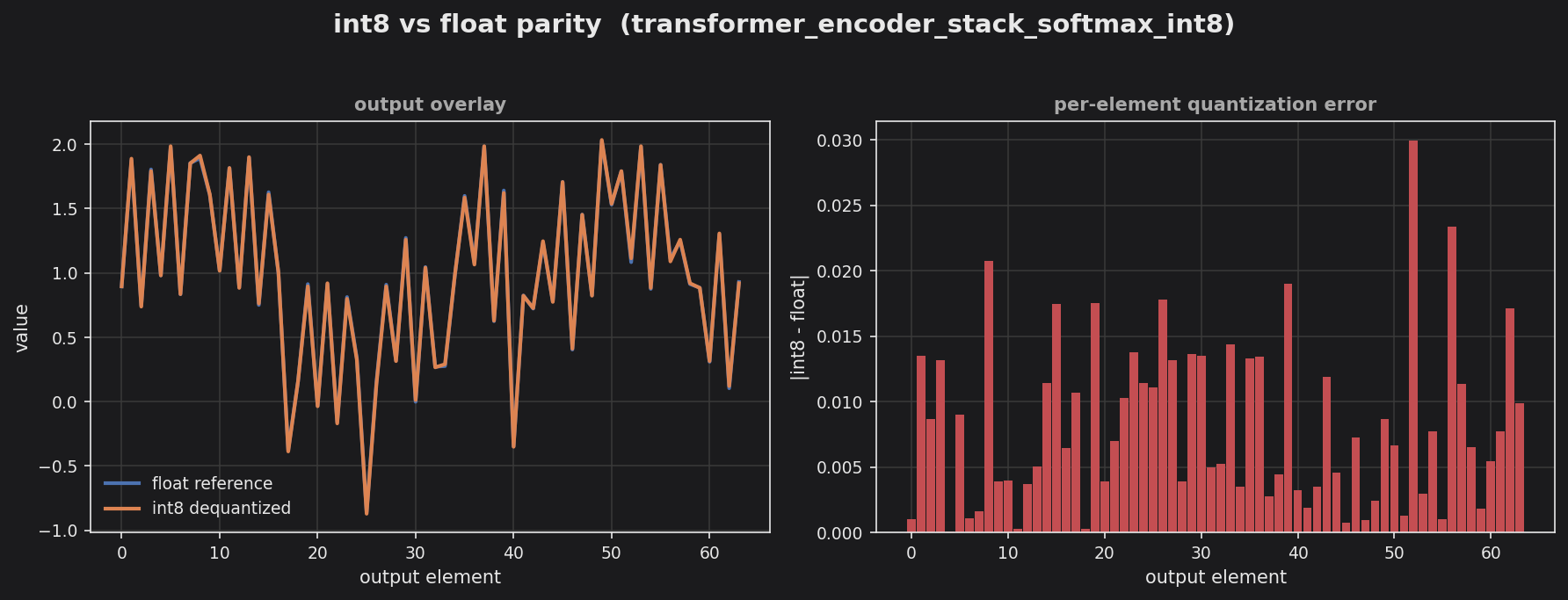

MobileNetV2-shaped pipeline (int8) — logit parity vs the float reference.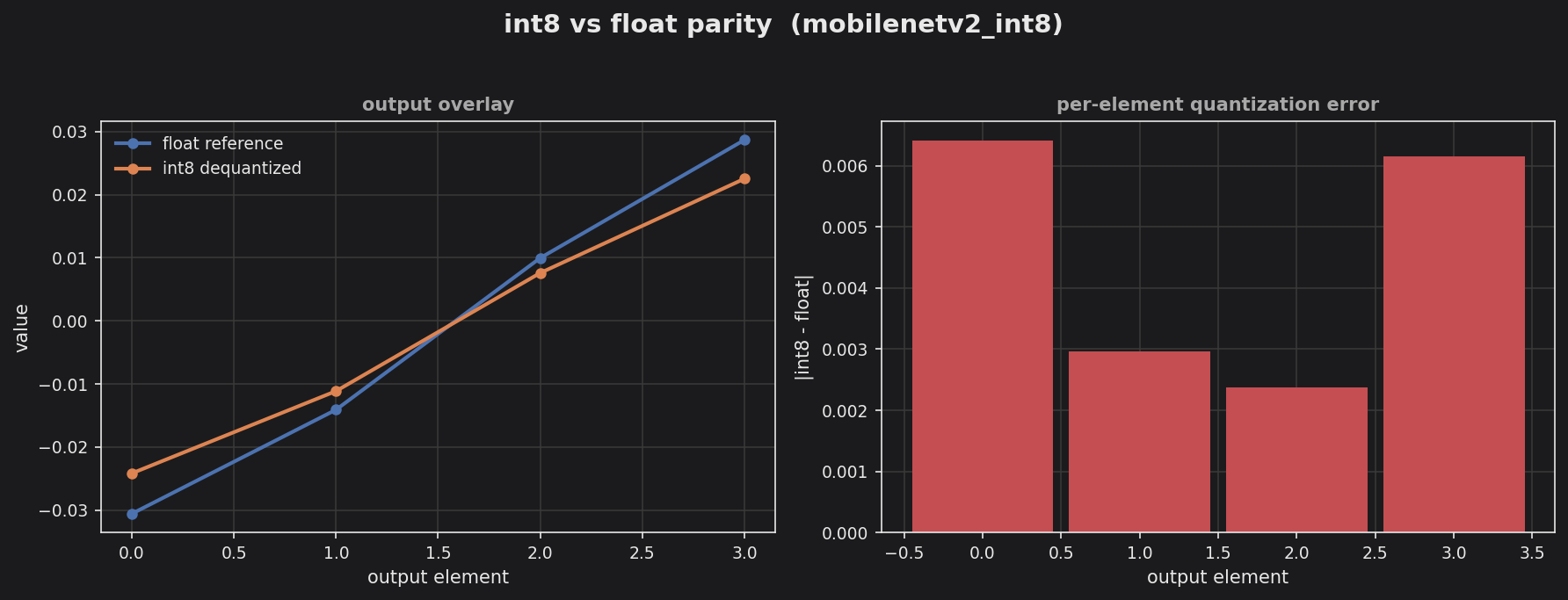

Mixture-of-Experts

int8 MoE regime routing — a top-1 router partitions the input domain into three regimes; one of three linear experts runs per inference (color blocks = the routing map).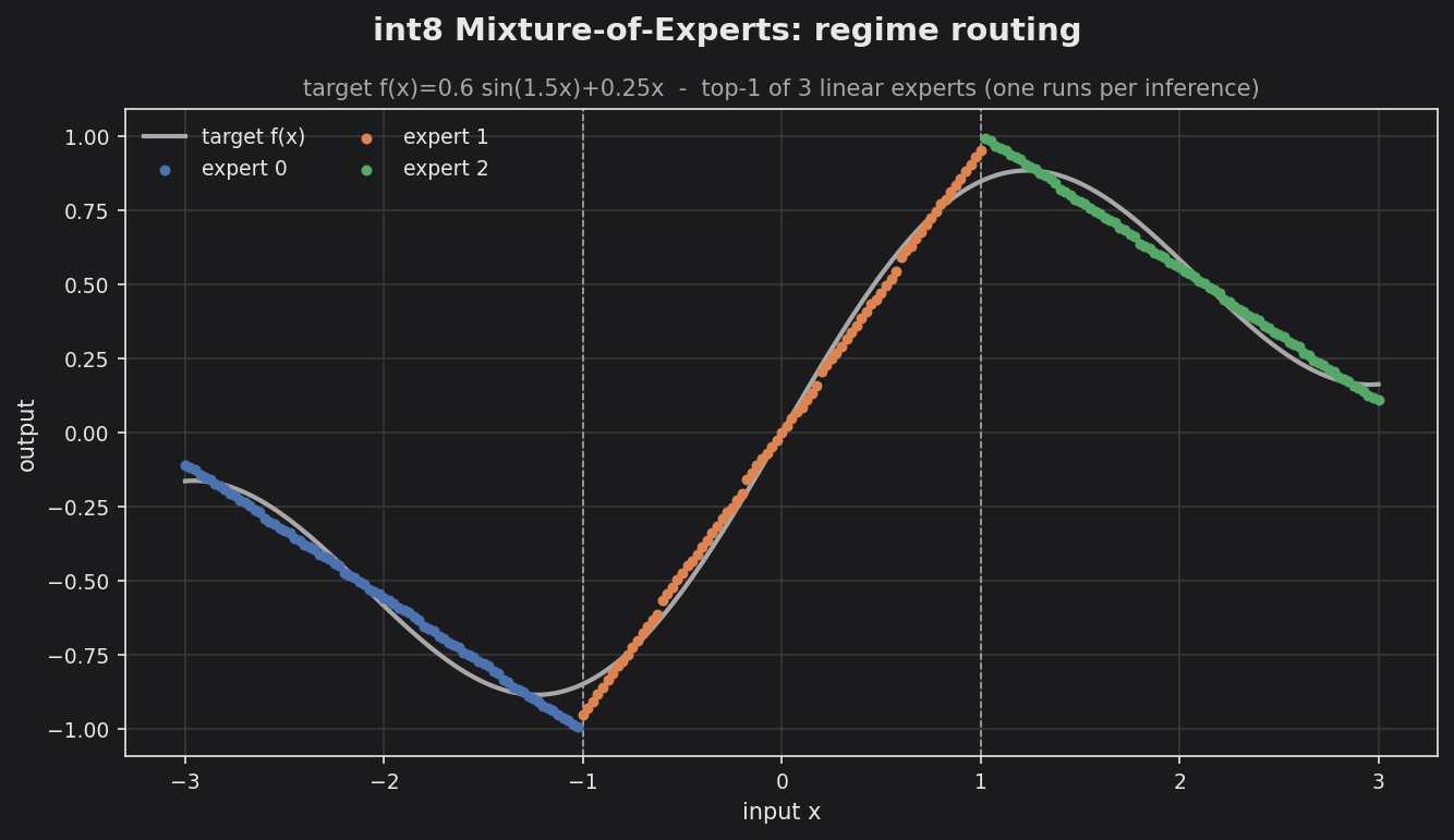

UCI dataset solutions

End-to-end examples on real (or documented-synthetic) UCI datasets — see the UCI Dataset Capability Report for which example uses which dataset.

Iris — Q16.16 MLP (4→8→3) species classifier; training loss, test confusion, petal-space predictions.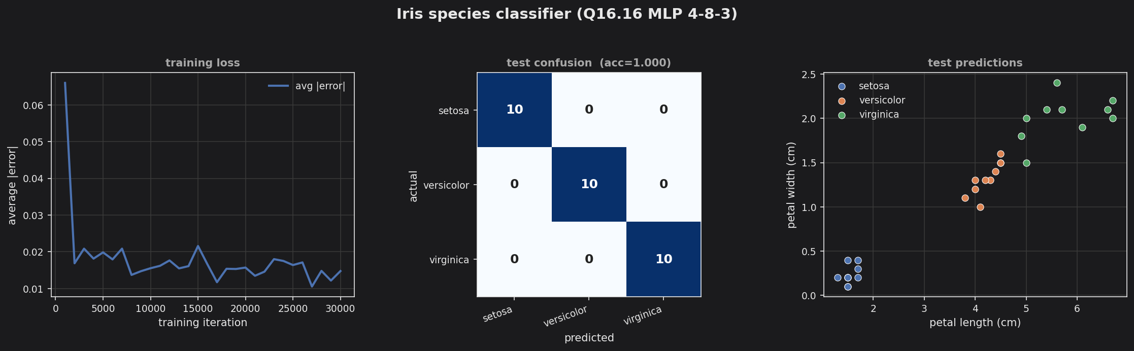

Energy Efficiency — Q16.16 MLP (8→16→2) regression of building heating/cooling load; predicted vs actual.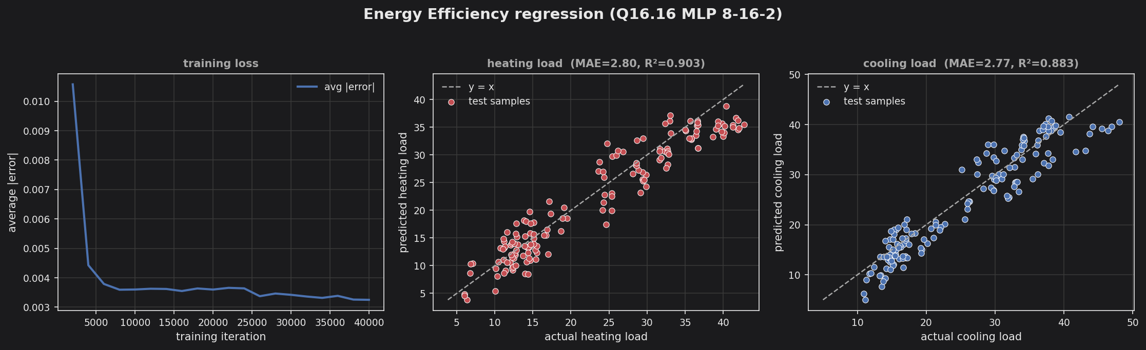

Optical digits — Q16.16 MLP (64→32→10) on 8×8 handwritten-digit bitmaps; loss + 10×10 confusion.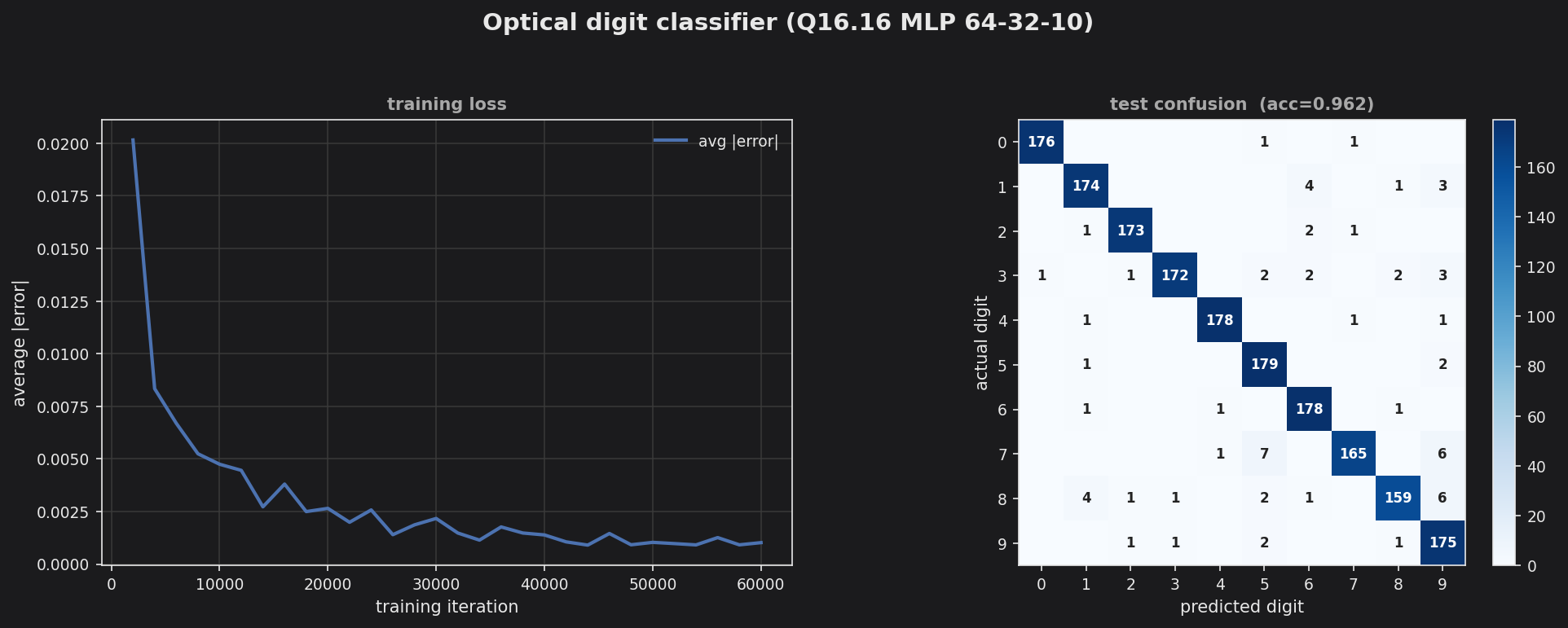

Human activity recognition — recurrent LstmNeuralNetwork (3→16→4) over tri-axial accelerometer windows.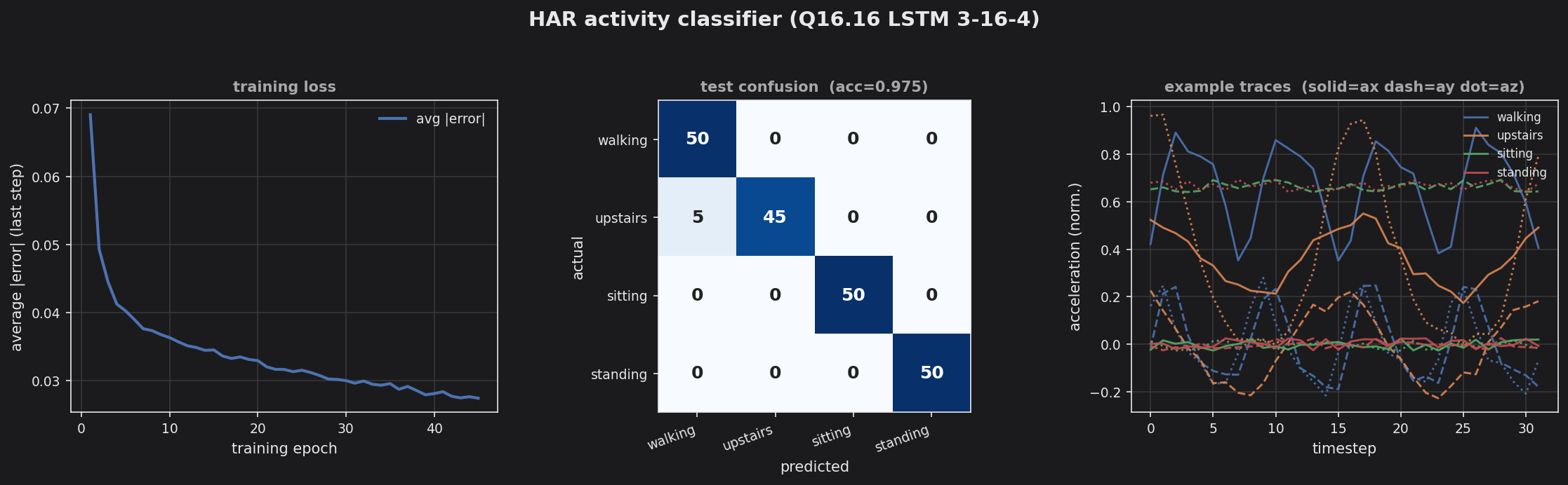

Japanese Vowels — recurrent ElmanNeuralNetwork (12→16→9) speaker ID; trained offline in float, then swept across fixed-point formats. Q8.8 matches double precision at 4× smaller weights.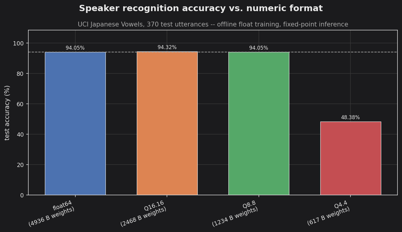

Gas sensor array drift — MLP (128→32→6) trained on batch 1; accuracy decays across later batches as sensors drift.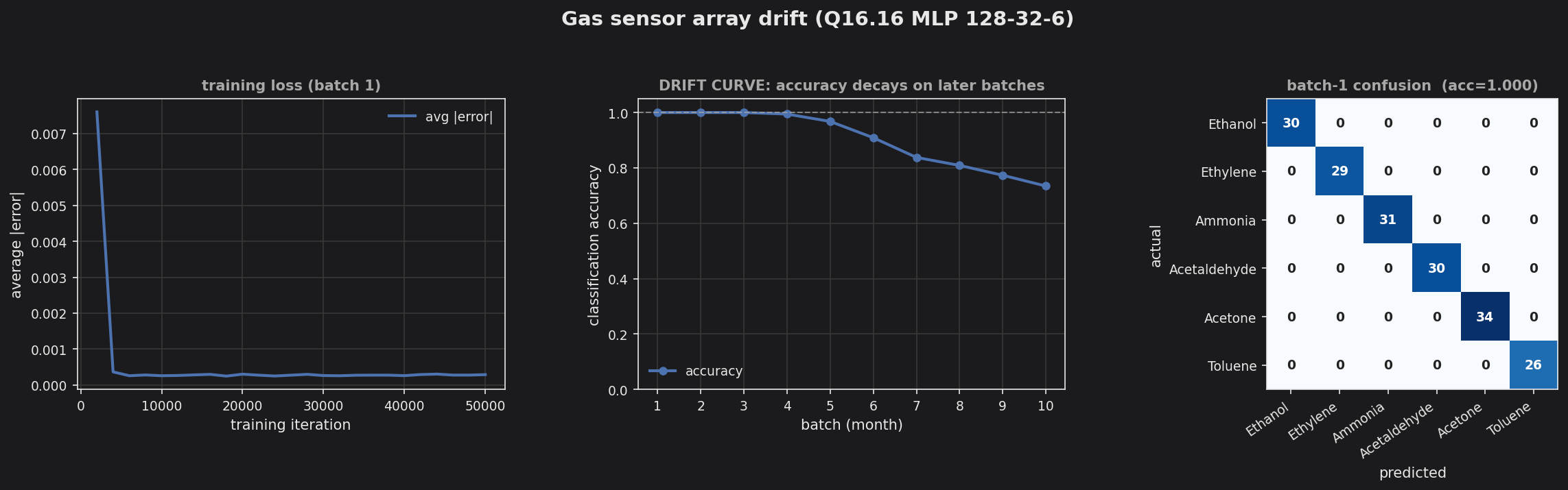

Air quality forecasting — recurrent LSTM (1→16→1) one-step-ahead hourly pollutant forecast.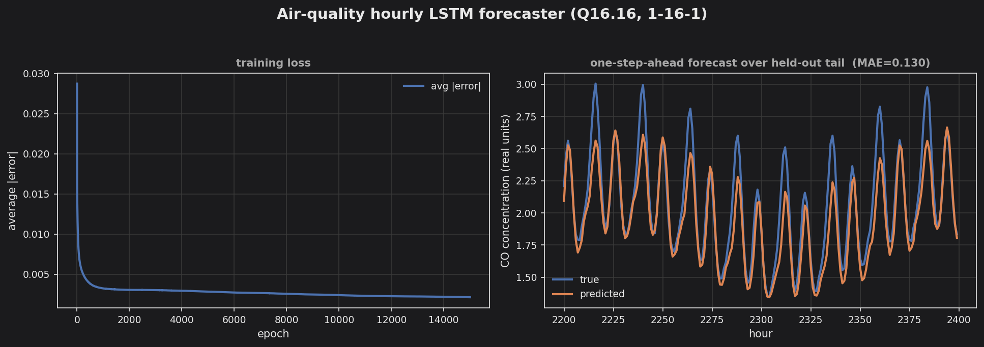

Cost & performance

KWS pipeline per-layer cost — compute cost + stacked weight/activation footprint per layer.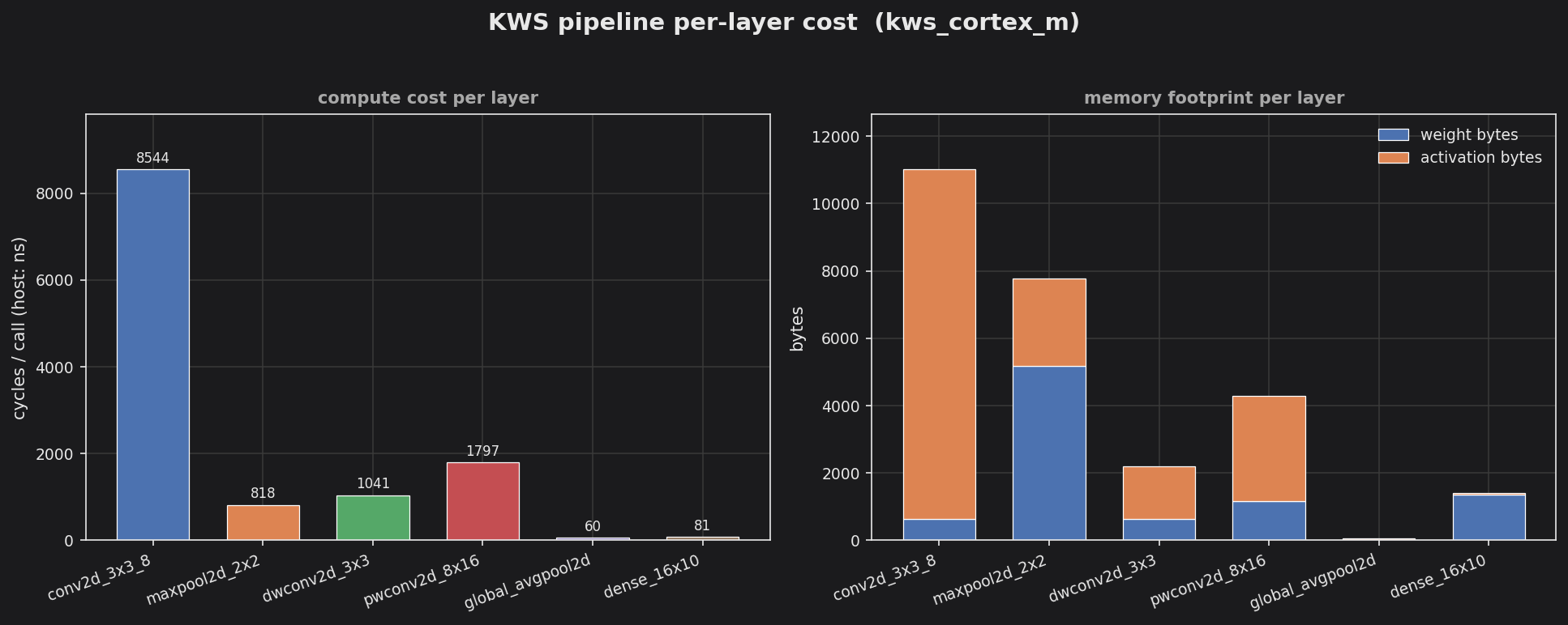

SIMD backends — int8 QConv2D / QDense throughput across backends (output checksum identical — bit-exact).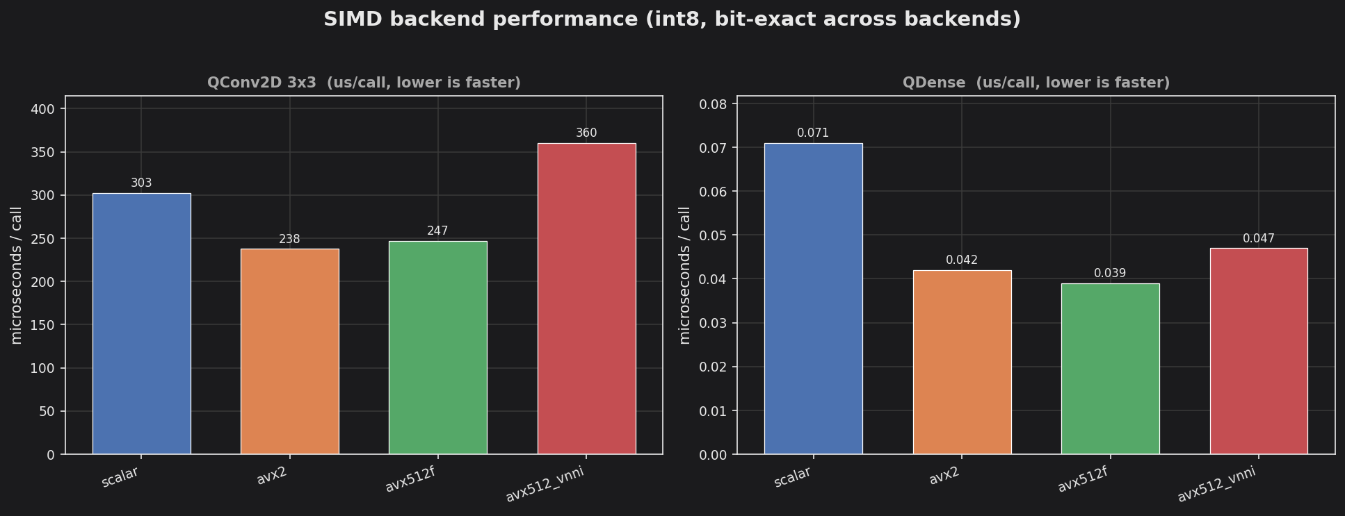

Applications

XOR decision surface — PyTorch-trained weights, pure-integer TinyMind inference; learned boundary as a heatmap.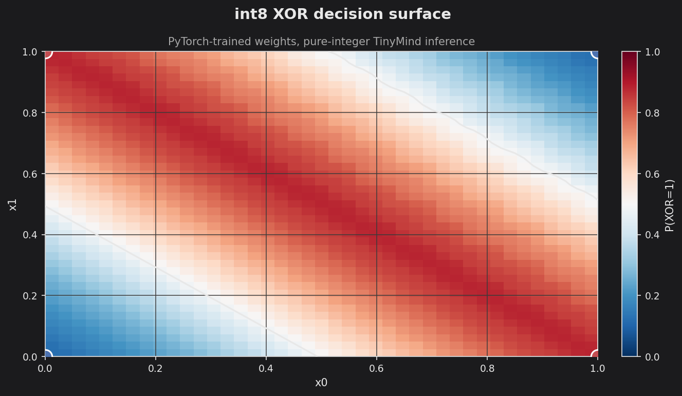

Predictive maintenance — training loss + test confusion matrix (machine-failure classifier).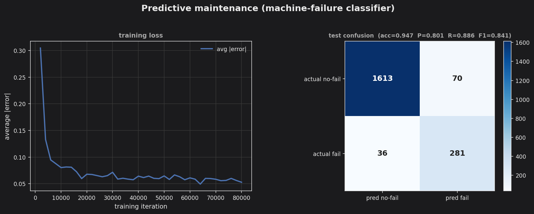

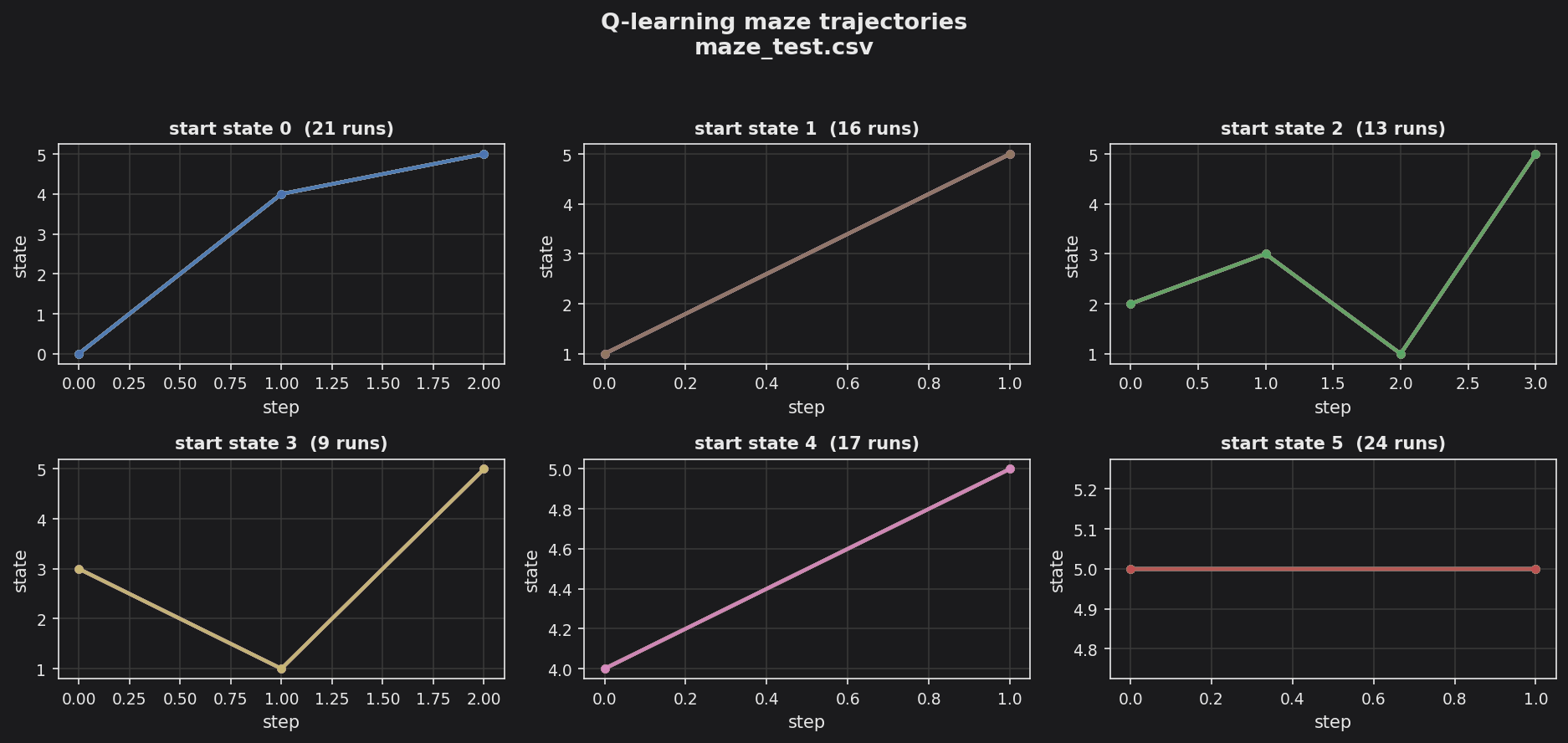
Q-learning maze — per-start-state navigation trajectories.